admin
admin
Today, I want to explain to you one of the most important and useful Excel functions for everyday work VLOOKUP. Whether you’re a student managing your marks, a shop owner tracking your sales, or someone working in an office with loads of data, this function can make your life easier. Excel is already a very helpful tool for small businesses and individuals alike and learning how to use VLOOKUP in Excel can boost your productivity and confidence.
What is VLOOKUP in Excel?📌
VLOOKUP stands for Vertical Lookup. That means Excel will search for a specific value vertically in the first column of a range and then return a value from the same row but from a different column that you specify.
Think of VLOOKUP like a super-fast finder tool. Instead of manually checking a big table to find one price, name, or value—you can ask Excel to do it for you automatically. And it’s super simple once you understand the basics.
For example: You have a product code, and you want to know its price. VLOOKUP will look down the product code column, and when it finds the code, it will give you the price from the same row.
🤔 Why Should You Use VLOOKUP?
✅Running a grocery store and want to pull product prices using the item code.
✅Managing employee data and want to search for someone’s department using their ID.
✅Working with student reports and want to quickly find a student’s grade.
Instead of scrolling through 100s of rows, just use VLOOKUP.
VLOOKUP helps you:
⏱️Save time
❌Avoid mistakes
⚙️Automate repetitive tasks
💼Look more professional
Understanding the VLOOKUP Formula🔍
Here is the formula syntax
=VLOOKUP(lookup_value, table_array, col_index_num, [range_lookup])
Let’s break it down:
lookup_value: What you’re searching for (e.g., product code).
table_array: Where to search (your data table).
col_index_num: From which column to return the result.
[range_lookup]: Use FALSE for exact match (always recommended for beginners).
Always use FALSE to get accurate results.
Example 01: Sales Count Lookup
Imagine you run a small shop. You have a sales report:
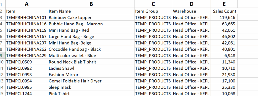
Now, you want to know how many sale count of TEMPBHHCHINA429
Your VLOOKUP Formula Breakdown is =VLOOKUP(A09,A:E,5,)
🔍 What Each Part Means:
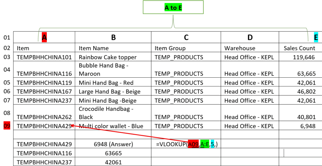
A09 = The value you want to look up.
👉 For example: an Item Code like"TEMPBHHCHINA429".A:E = The range where Excel should search.
👉 It starts from column A (Item) to column E (Sales Count).5 = The column number in the selected range to return data from.
👉 Column A is 1, B is 2, …, E is 5.
So if you want to get Sales Count, use5.
If you want Item Name, use2.FALSE = This tells Excel to look for an exact match (always use
FALSEwhen working with unique IDs or text).
Example 02: Product Price List
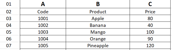
You can create another table with just the product code, and use this formula: Need to find the price of Banana=VLOOKUP(A4, A:C, 3)
Common VLOOKUP Mistakes⚠️
1. Wrong Column Placement
The lookup value must be in the first column of your table range.
If it’s not, VLOOKUP won’t find it—no matter how close your formula is!
Wrong Example:
You want to look up an employee name using their ID, but your table starts with names and the IDs are in the second column.=VLOOKUP("E102", B2:C6, 2, FALSE)❌ This won’t work!
Correct Way:
Always make sure the ID (the lookup value) is the first column:=VLOOKUP("E102", A2:C6, 2, FALSE)✅
Tips to Be a VLOOKUP Pro💡
Turn your data into an Excel Table (Ctrl + T) for better dynamic formulas.
Combine VLOOKUP with DROP-DOWN lists for interactive dashboards.
Use conditional formatting to highlight values found by VLOOKUP.
Make your data consistent: remove duplicates and blank rows.
Use Named Ranges to make your formulas easier to understand.
When to Avoid VLOOKUP❌
VLOOKUP only searches from left to right. If your lookup value is not in the first column, it won’t work.
Instead, try:
INDEX +MATCH
XLOOKUP (available in Excel 365)
FILTER() for multiple results
These functions offer more flexibility than VLOOKUP.
VLOOKUP is simple but powerful. With this one function, you can search through tables, match values, and automate tasks that would take hours manually. Start practicing today and take one more step to becoming a true Excel pro! 💪