admin
admin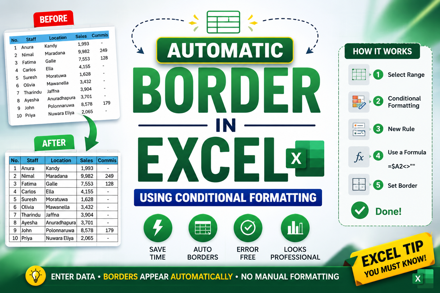
Have you ever noticed that every time you enter new data into an Excel table, you have to manually add borders?
If you work with sales reports, employee lists, invoices, inventory records, or customer databases, this can become repetitive and time-consuming.
The good news is that Microsoft Excel allows you to create automatic borders using Conditional Formatting. Once it’s set up, Excel will automatically draw borders whenever you enter data into your worksheet.
No VBA. No Macros. No complicated formulas.
Let’s learn how to do it.
Why Use Automatic Borders?
Using automatic borders has several advantages:
- Saves time when entering data
- No need to format each new row manually
- Keeps worksheets neat and professional
- Perfect for reports and dashboards
- Great for inventory, sales, attendance, customer lists, and financial records
- Works without VBA or macros
Download the Practice Workbook
Before we begin, download the sample Excel workbook below and follow along with each step in this tutorial.
This practice file contains a simple employee sales table that we’ll use to demonstrate how to automatically add borders in Excel using Conditional Formatting.
By practicing with the sample workbook, you’ll be able to see the automatic border effect in real time. As you add new employee records, Excel will automatically apply borders to the newly entered datawithout any manual formatting.
Let’s get started and build this useful Excel trick together!
Step 1 – Select the Range
First, highlight the entire area where you expect to enter data.
Don’t select only your existing records.
Instead, select additional blank rows so Excel will continue applying borders as future data is entered.
For example, if your current table ends at row 10, you might select rows 2 through 500.
This ensures that every future record automatically receives borders.
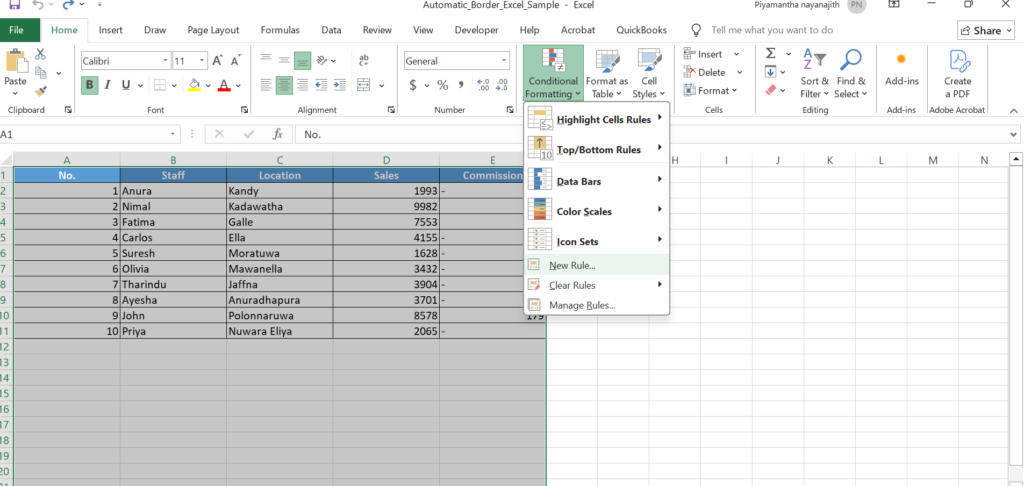
Step 2 – Open Conditional Formatting
Now follow these steps:
Home → Conditional Formatting → New Rule
A new window will appear with several rule options.
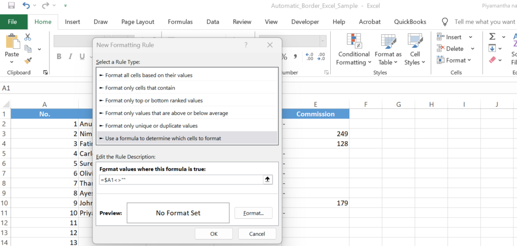
Step 3 – Choose “Use a Formula”
Select
Use a formula to determine which cells to format
This option tells Excel to check whether a row contains data before applying the formatting.
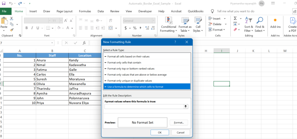
Step 4 – Enter the Formula
If your data starts in Column A, enter this formula:
=$A1<>””
What this formula means:
- If cell A2 contains data
- Apply the selected formatting
- If A2 is empty
- Don’t apply any border
As soon as you type something into Column A, the entire row will receive borders.
Step 5 – Add the Border
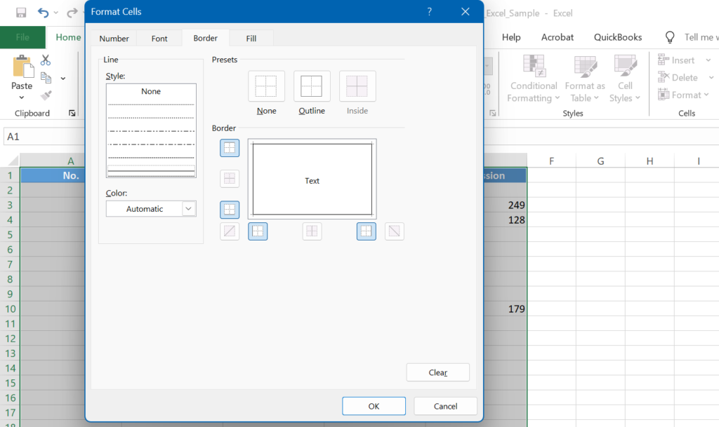
Click – Format, Then go to the Border tab. Choose
- Outline Border
or select All Borders, depending on your preferred table style.
Click OK.
Then click OK again.
Your automatic border rule is now complete.
Automatic borders may seem like a small Excel feature, but they can make a big difference in your daily work. Instead of manually adding borders every time you enter new data, you can let Conditional Formatting do the work automatically.
Whether you’re managing sales reports, inventory, employee records, customer databases, invoices, or financial reports, this simple Excel trick will save you time, reduce formatting errors, and keep your spreadsheets looking clean and professional.
To get the best results, download the practice workbook and follow along with this tutorial step by step. I’ve also shared a practice video that demonstrates the entire process from start to finish. Watch the video, practice the steps yourself, and repeat them until you feel confident using this technique in your own Excel projects.
If you found this tutorial helpful or learned something new today, please share this article with your friends, colleagues, or classmates who use Excel. You might help someone save hours of repetitive work.
💬 Tag someone who always spends time formatting Excel sheets manually-they’ll definitely appreciate this trick!
Don’t forget to bookmark this page and follow us for more Excel tutorials, productivity tips, formulas, Conditional Formatting tricks, dashboards, and Microsoft Excel guides. New tutorials are published regularly to help you work smarter and become an Excel expert.
Happy Learning! 🚀