admin
admin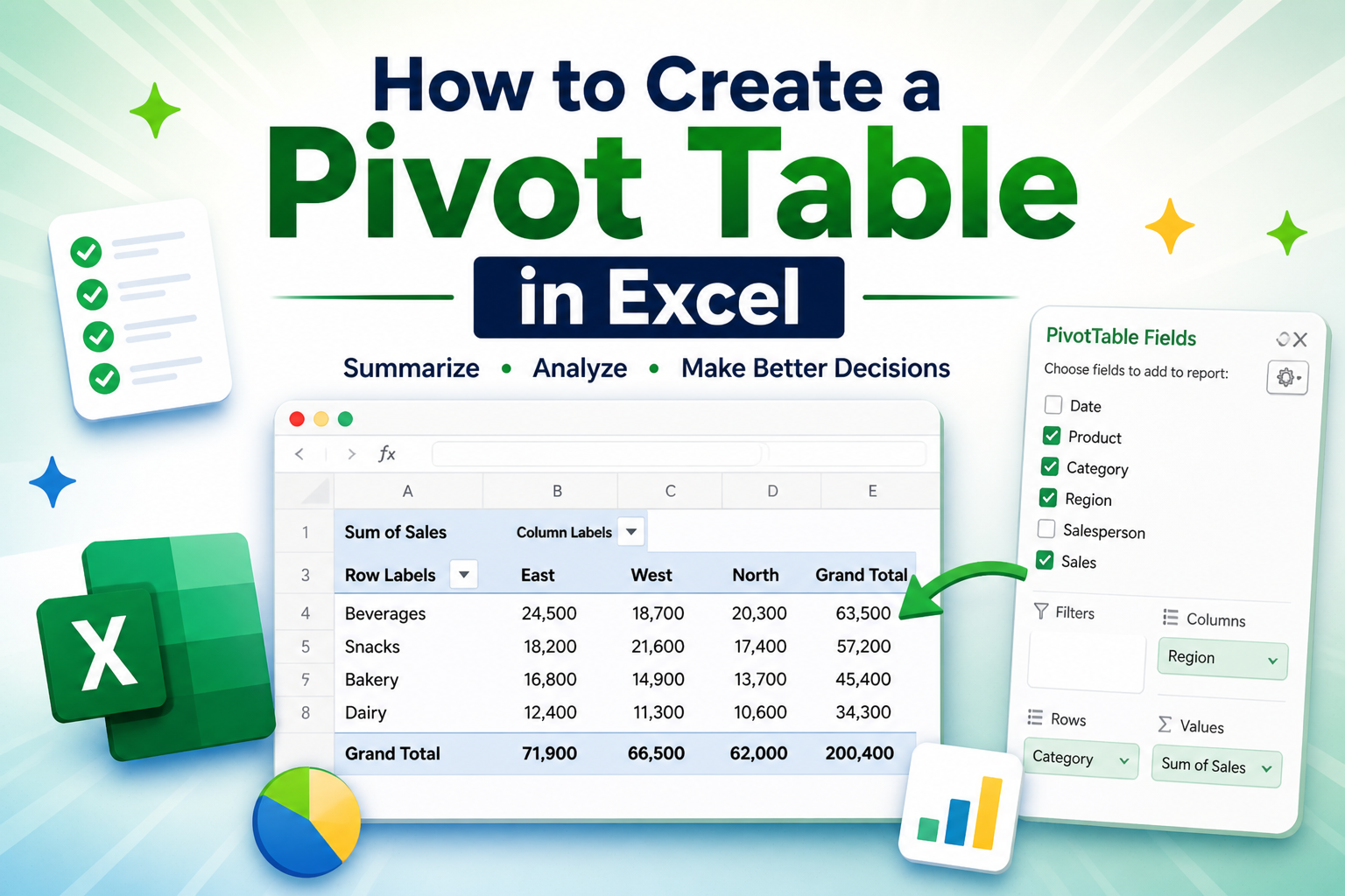
Introduction
These days, everything runs on data.Whether it’s sales, inventory, or even a small online business, we’re constantly dealing with numbers. But the real challenge isn’t collecting data,it’s understanding it quickly.
If someone asks you:
👉 “Which product is selling the most?”
👉 “Which region is performing best?”
You don’t want to scroll through thousands of rows trying to figure it out.
That’s exactly where Microsoft Excel becomes powerful – especially with tools like:
- Pivot Table in Excel
- Power Pivot in Excel
In this guide, I’ll walk you through everything in a simple way – no complicated explanations, just practical understanding you can actually use.
📌 What Is a Pivot Table?
A Pivot Table is basically a smart summary tool inside Excel. It takes a large set of data and turns it into something simple and meaningful – in just a few clicks.
Instead of manually calculating totals or writing formulas, Excel does all the work for you.
💡 Think of It Like This
Imagine you have a sales sheet with thousands of rows.
Each row has:
- Product
- Region
- Sales amount
Now someone asks:
👉 “What’s the total sales by region?”
Doing this manually would take a lot of time.
With a Pivot Table?
👉 You get the answer in seconds.That’s the power.
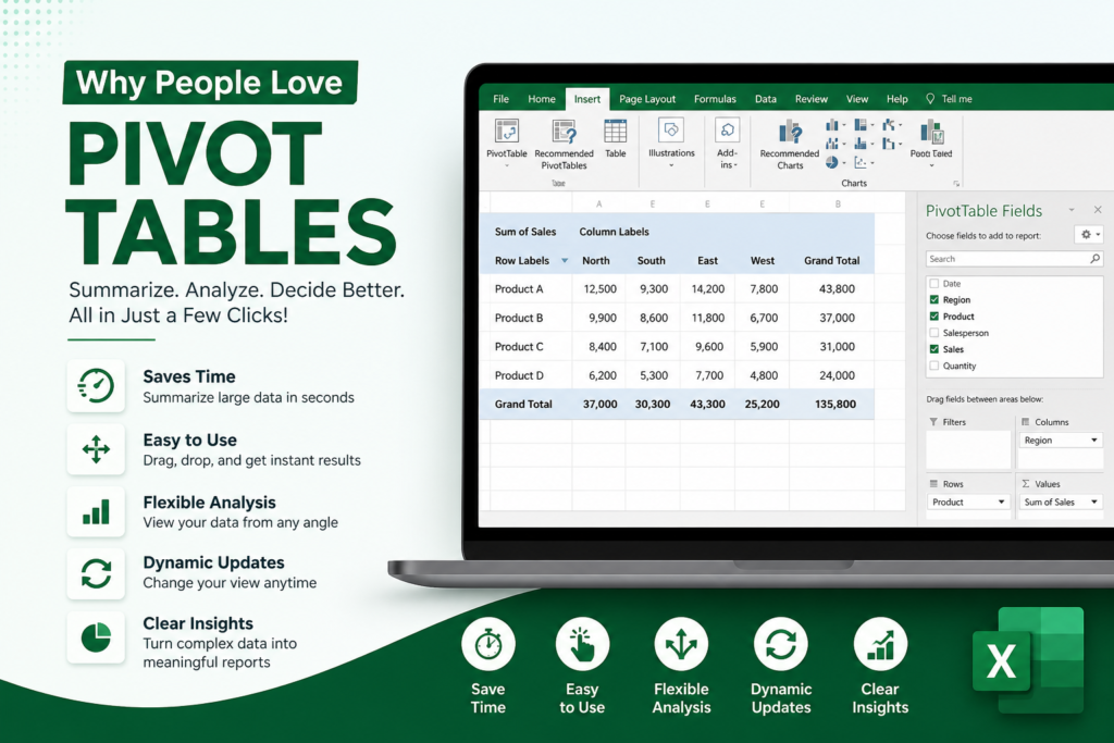
🚀 Why People Love Pivot Tables
Once you start using Pivot Tables, it’s hard to go back.
You save a lot of time
You can change your report instantly
No need to remember complex formulas
It’s perfect for real work (not just learning)
🛠️ How to Create a Pivot Table (Step-by-Step)
Don’t worry, this is much easier than it sounds.
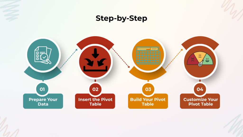
✅ Step 1: Prepare Your Data
Before anything, make sure your data is clean.
That means:
- Each column has a name (like Product, Sales, Date)
- No empty rows in between
- Each row is one record
👉 If your data is messy, your Pivot Table will also be messy.
✅ Step 2: Insert the Pivot Table
- Click anywhere inside your data
- Go to the Insert tab
- Click PivotTable
- Choose “New Worksheet”
- Click OK
That’s it — Excel will create a blank Pivot Table for you.
✅ Step 3: Build Your Report
Now comes the fun part.
You’ll see a panel with your column names.
You just drag and drop:
- Put Region → Rows
- Put Product → Columns
- Put Sales → Values
And instantly — your report is ready.
No formulas. No stress.
📊 Real-Life Example (Important)
Let’s make this practical.
If you’re managing inventory or sales (like most businesses):
You can use Pivot Tables to:
- Track best-selling products
- Check slow-moving items
- Analyse monthly sales
- Compare regions
👉 This is exactly how companies make decisions.
In this tutorial, we are using a full-month dataset to simulate real business data, making it easier to understand how Pivot Tables work in real-world scenarios.📥 I’ve included a sample Excel sheet for you. Download it and follow each step with me, you’ll learn much faster by doing.
✅ Example 1 – Sales by Product & Region
🎯 What We Are Trying to Do
We want to create a summary like this:
- Show each product
- Break it down by region
- Calculate total sales
🎥 Here is my screen recording. Watch it carefully, then repeat the same steps on your side. That’s the fastest way to learn Pivot Tables.
📊 Example 2: Monthly Total Sales (Pivot Table)
Now let’s look at another useful scenario.
Instead of analysing by product or region, this time we want to answer:
👉 “What is the total sales for each month?”
🎯 Goal
- Group sales by month
- Calculate total sales per month
🎥 Monthly Total Sales (Practice With Me)
For this example, we don’t need to repeat everything again.
👉 Step 1 to Step 3 are exactly the same as the previous example.
▶️ Watch & Practice
🎥 Here is my screen recording. Watch how I build the Pivot Table, and then try it yourself step by step.
🧩 Key Setup for This Example
Once your Pivot Table is ready, just change the fields like this:
Date  → Rows
Sales → Values (Sum)
Sales → Values (Sum)
🎯 Practice Task (Your Homework)
By now, you’ve learned the basics of how Pivot Tables work — and more importantly, how powerful they can be.
But here’s the truth:
👉 You won’t really understand Pivot Tables just by reading.
👉 You need to try it yourself.
🧩 Task 1: Sales by Salesperson
Create a Pivot Table to find:
👉 Who generated the highest sales?
Salesperson → Rows
Sales       → Values (Sum)
💡 This will give you a clear breakdown of total sales for each salesperson.
🧩 Task 2: Category Performance
Create a Pivot Table to find:
👉 Which category is performing the best?
Category → Rows
Sales    → Values (Sum)
💡 This helps you understand which product category is driving the most revenue.
🚀 Don’t Just Read — Do It
Take a few minutes and actually build these Pivot Tables in Excel.
- Try dragging fields yourself
- Change positions and see what happens
- Explore different views
👉 This is where real learning happens.
Once you’re done:💬 Take a screenshot of your Pivot Table and share it in the comments.